Bayesian Stats Will Teach You How to Hide a Geocache
This is an example of a project that I worked on using Bayesian statistics
What is a Geocache?
You may have heard about Bayesian statistics, but have you heard of Geocaching? In this post I’ll explain to you how my friend Drew Millane and I designed a Bayesian model to explore what kind of geocache will get you the most favorite points, but first I need to explain to you what a geocache is.
Geocaching is the world’s largest treasure hunt. The first geocache was hidden on May 3rd, 2000 and since then over 3 million more geocaches have been hidden across 191 different countries and all 7 continents. There are over 300,000 cache owners in the world. In 2020 a geocache tagged along for a ride to Mars with NASA’s Perseverance rover and landed in the Jezero Crater in early 2021, marking the first interplanetary geocache. With such a buzz about geocaching, it is only natural to wonder what makes a good geocache.
No two geocaches are the same. Some are placed in difficult-to-reach places (see the geocache on Mars above), others are easy to get to but craftily hidden. A cache’s “Terrain” rating indicates the physical effort that will be needed to get to the cache while a cache’s “Difficulty” rating indicates the amount of effort that will go into solving or finding the cache. Some geocaches are as large as a boulder, others are as small as a thimble. When a geocacher finds a geocache they have the option to grant that cache a “favorite”, similar to a “like” on social media. The goal of our analysis is to determine whether a cache’s Terrain or Difficulty rating affects the number of favorites it receives.
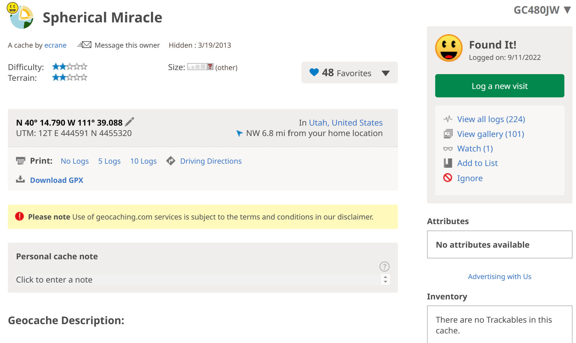
Above is an example of a geocache page. This cache has a Terrain and Difficulty rating of 2, is size “Other”, and has received 48 favorites at the time of posting
What makes a cache popular?
Now with a bit of background info, the next logical question to ask is “What makes a geocache popular”? Fantastic question. Obviously if you are going to spend the effort to hide a cache you would like it to be found and for other geocachers to enjoy it. Drew and I decided to train a Bayesian model on some geocaching data to find an answer to that question.
The data
Our model was trained on data from 144,000 geocaches from the states of Utah and California. We used the Difficulty, Terrain, and number of Favorites.
Our model
I may spend more time on another post explaining more about Bayesian statistics but for now I’ll explain our model as if you already have a base level understanding of how to build a Bayesian model.
We wanted to train our model based on the number of Favorites as the target variable, and since the number of Favorites is a count variable we decided to use a Poisson likelihood. All together then that makes nine groups for Terrain and Difficulty (since Terrain and Difficulty are measured from 1-5, incrementing by .5) each. Our model specifies a rate parameter for each group taken from a Gamma distribution. We then imposed priors on alpha and beta for each group, which resulted in a grand total of 27 parameters to be estimated.
We specified the priors for alpha and beta in a way that would result in an expected count of approximately five favorites for each group. This was a bit of a shot in the dark, we just assumed each group would have around the same number of favorites.
Below is our actual model that we created.
\[y_{i} \mid \lambda_{i} \sim \text{Pois}(\lambda_{i})\] \[\lambda_{i} \mid \alpha_{i}, \beta_{i} \sim \text{Gamma}(\alpha_{i},\beta_{i})\] \[\alpha_{i} \mid c, d \sim \text{Gamma}(c,d)\] \[\beta_{i} \mid e, f \sim \text{Gamma}(e,f)\] \[y_i \text{is the number of favorites a given cache has received}\] \[\text{Prior: c = 5, d = 1, e = 1, f = 1 }\]For fun, we used a PPL for sampling and then we also wrote out our own sampler by hand. We used Stan for a PPL. Using a PPL made setting up our Bayesian model very simple, it abstracted away a lot of the complex math for us. However, in terms of computational time it was much slower than our by-hand sampler. Our by-hand sampler only took about 55 seconds to run whereas Stan took around 442 seconds to run each time. Just another example of how being a math ninja can pay off. ;)
By-hand analysis
We decided we would use a slice sampling method (If you want a post dedicated to the intricacies of slice sampling itself, shoot me an email), so to do that we had to write out our complete joint posterior density and from there derive the full conditionals of $\lambda$, $\alpha$, and $\beta$ for each group.
\(p(\lambda_{i} \mid \alpha_{i}, \beta_{i}, c, d, e, f, y_{1}, ...,y_{m}) \propto p( y \mid \lambda_{i})p(\alpha_{i} \mid c,d)p(\beta_{i} \mid e,f)\) \(\quad \prod_{i=1}^{n}\prod_{j=1}^{m}\frac{\lambda^{y_{ij}}e^{-\lambda_{i}}}{y_{ij}!} \frac{\beta_{i}^{\alpha_{i}}}{\Gamma(\alpha_{i})}\lambda_{i}^{\alpha_{i}-1}e^{-\beta_{i}\lambda_{i}}\frac{d^{c}}{\Gamma(c)}\alpha_{i}^{c-1}e^{-d\alpha_{i}}\frac{f^{e}}{\Gamma(e)}\beta_{i}^{e-1}e^{-f\beta_{i}}\)
To make that easier we just took the log of the joint and we got the following full conditionals
\((\lambda_{i} \mid \cdot) = \sum_{j=1}^{m}[y_{ij}\log(\lambda_{i})] - m\lambda_{i} + (\alpha_{i}-1)\log(\lambda_{i}) - \beta_{i}\lambda_{i}\) \((\alpha_{i} \mid \cdot) = \alpha_{i}\log(\beta_{i})-\log(\Gamma(\alpha_{i}))+\alpha_{i}\log(\lambda)+(c-1)\log(\alpha_{i})-d\alpha_{i}\) \((\beta_{i} \mid \cdot) \sim \text{Gamma}(\alpha_{i}+e,\lambda_{i}+f)\)
We then used the following algorithm to actually get draws from our distributions
Algorithm 1: By Hand Sampler
- Choose initial values for all $\lambda$, $\alpha$, and $\beta$
- For 10,000 Draws:
- For Each group:
- Sample $\beta$ from a Gamma
- Slice Sample the full conditional of $\alpha$
- Slice Sample the full conditional of $\lambda$
- For Each group:
Diagnostic plots
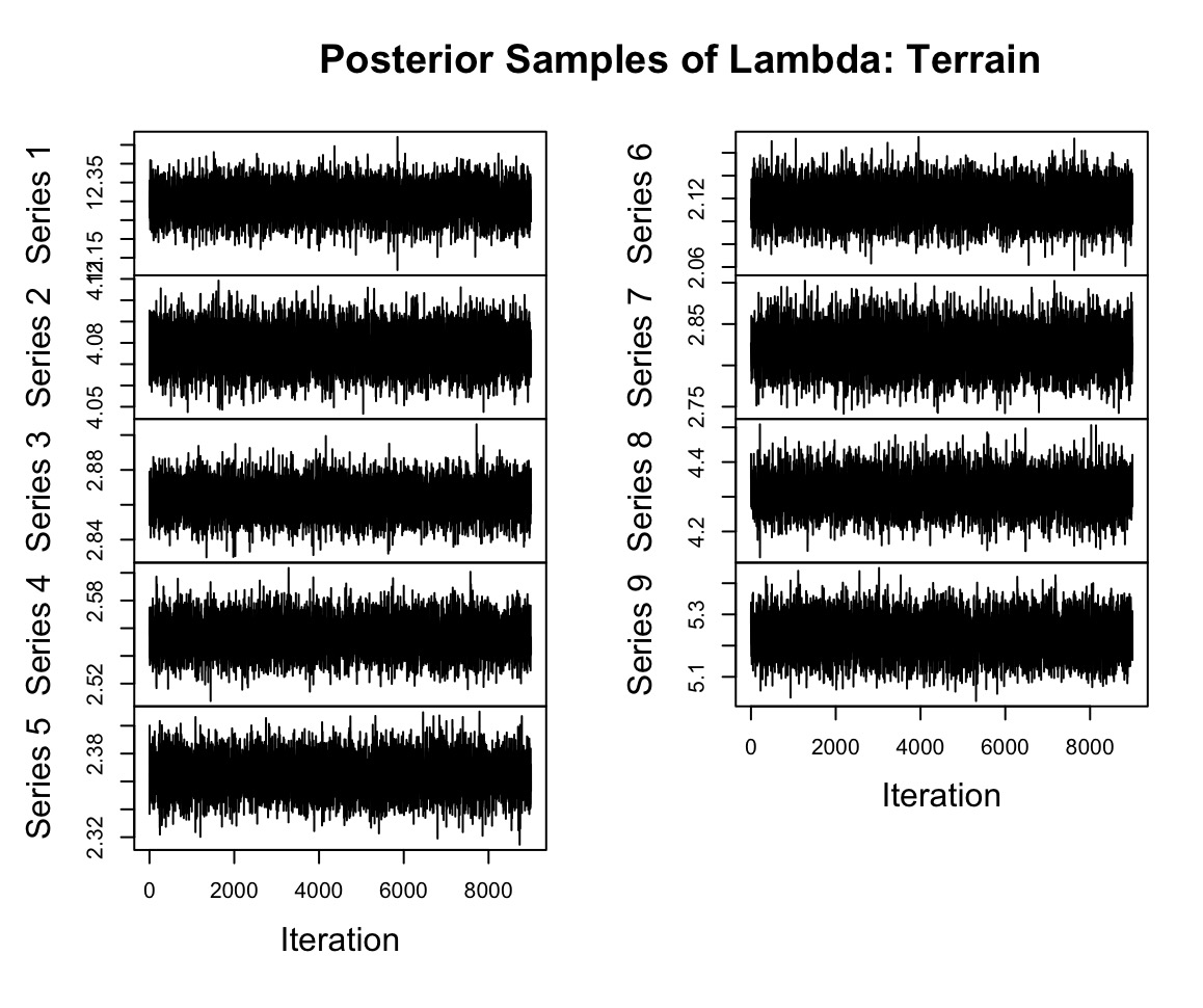
Now to verify that our PPL worked well we looked at some diagnostic plots. Below are just some example trace plots to make sure our model was really exploring the space well. Because they look nice and thick and not thin and wiry we know that the PPL was effective.
The next diagnostic that we looked at was the effective sample size for each group. Because our samples we are drawing from the posterior distribution are technically correlated and not independent, we want to measure what the effective number of samples we are using for our analysis is. If that number is too low then we may need to devise a better sampling method. Below is a table of the effective sample size for each Terrain group.
| Lambda | Value |
|---|---|
| var1 | 8697.055 |
| var2 | 8931.027 |
| var3 | 9578.830 |
| var4 | 9000.000 |
| var5 | 9389.972 |
| var6 | 9792.548 |
| var7 | 8683.698 |
| var8 | 9000.000 |
| var9 | 9000.000 |
Around 9000 samples for each group is fantastic, so we really weren’t worried.
Comparing our samplers
Now we definitely trust our Stan sampler, so we wanted to compare between Stan and our by-hand sampler to see if they were giving us the same results. We did this to see if our results were within Monte Carlo error of each other. To do this we took samples from both samplers and by taking the differences between the two we were able to create confidence intervals. Each of these intervals below contain zero so we know that both of our samplers were giving us the same results.
Difference in PPL/By-hand estimation of mean favorites per group for Difficulty
| Difficulty Level | Lower Bound | Upper Bound |
|---|---|---|
| 1 | -0.0012 | 0.0005 |
| 1.5 | -0.0001 | 0.0003 |
| 2 | -0.0001 | 0.0003 |
| 2.5 | -0.0007 | 0.0003 |
| 3 | -0.0007 | 0.0006 |
| 3.5 | -0.0009 | 0.0014 |
| 4 | -0.0012 | 0.0017 |
| 4.5 | -0.0001 | 0.0049 |
| 5 | -0.0036 | 0.0019 |
Difference in PPL/By-hand estimation of mean favorites per group for Terrain
| Terrain Level | Lower Bound | Upper Bound |
|---|---|---|
| 1 | -0.0004 | 0.0020 |
| 1.5 | -0.0001 | 0.0004 |
| 2 | -0.0003 | 0.0002 |
| 2.5 | -0.0004 | 0.0003 |
| 3 | -0.0003 | 0.0005 |
| 3.5 | -0.0005 | 0.0004 |
| 4 | -0.0004 | 0.0010 |
| 4.5 | -0.0006 | 0.0023 |
| 5 | -0.0024 | 0.0010 |
Sensitivity of priors
You may have noticed my justification of the priors that we used earlier to be a little less than satisfactory. I don’t disagree, but just to be safe we tested how sensitive our model is to using different priors (spoiler alert: our model used so much data it didn’t even matter what our prior was).
To do this we tried using our model but with a crazy strong prior with c = 1000, d = 1, e = 1, f =1. Below is a table of the differences in mean favorites for each group as calculated by our original model and the model with the new prior. The differences are very small, so we just concluded that the prior wasn’t terribly important.
| Lower Bound | Upper Bound |
|---|---|
| 0.0004 | 0.0028 |
| 0.0003 | 0.0008 |
| 0.0011 | 0.0016 |
| 0.0023 | 0.0030 |
| 0.0028 | 0.0036 |
| 0.0056 | 0.0065 |
| 0.0081 | 0.0095 |
| 0.0166 | 0.0195 |
| 0.0148 | 0.0182 |
So, what kind of geocache is the best?
Below are density plots of the mean number of favorites for each group of Difficulty and Terrain. On both graphs, the two extremes of Difficulty and Terrain (highest and lowest ratings) have the most favorites. It’s also interesting to note that the distribution of each group almost never overlaps with the distributions of other groups, which implies that the Difficulty and Terrain rating of each geocache really does impact the number of favorites that each cache receives.
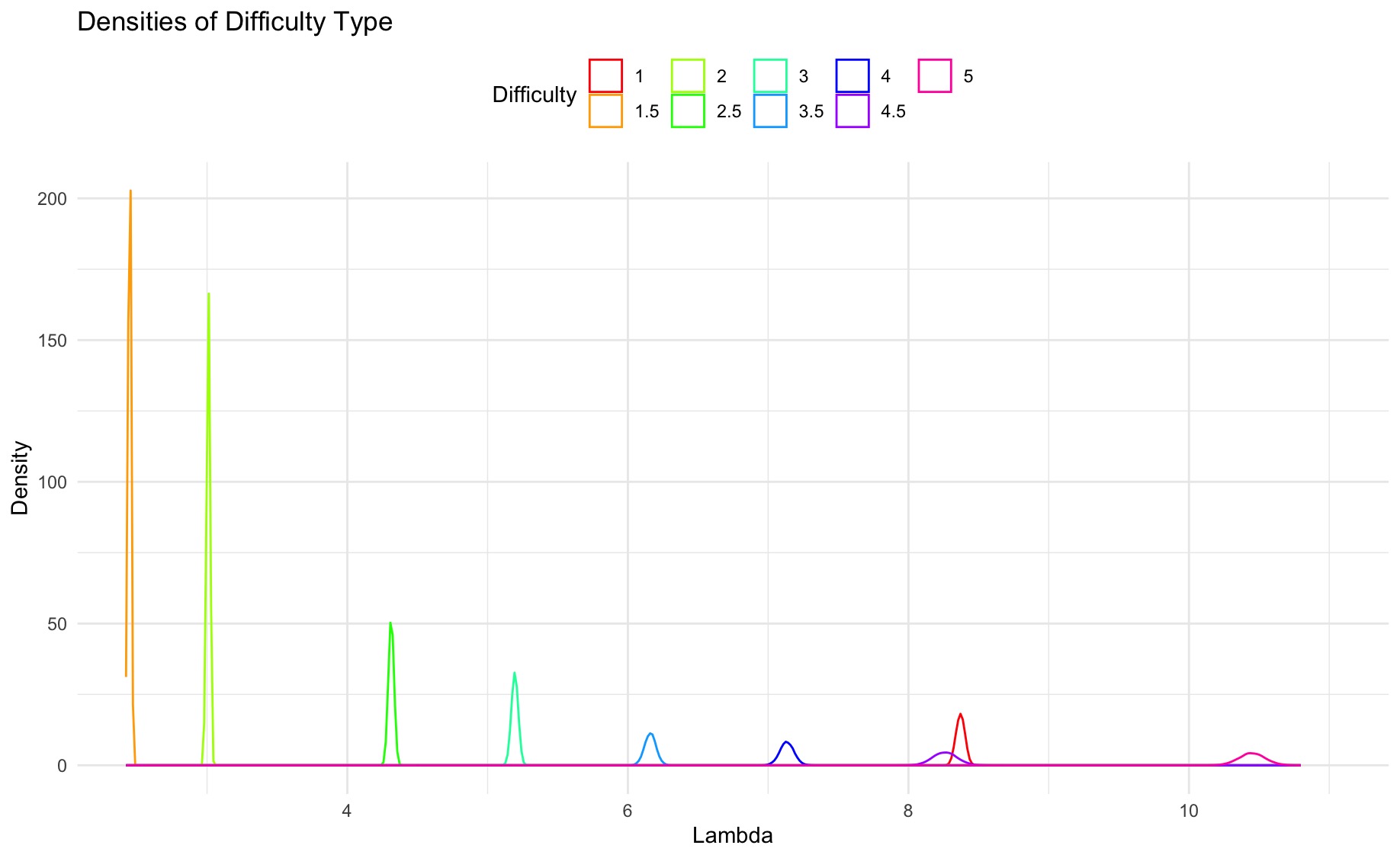
Densities of mean number of favorites by Difficulty rating
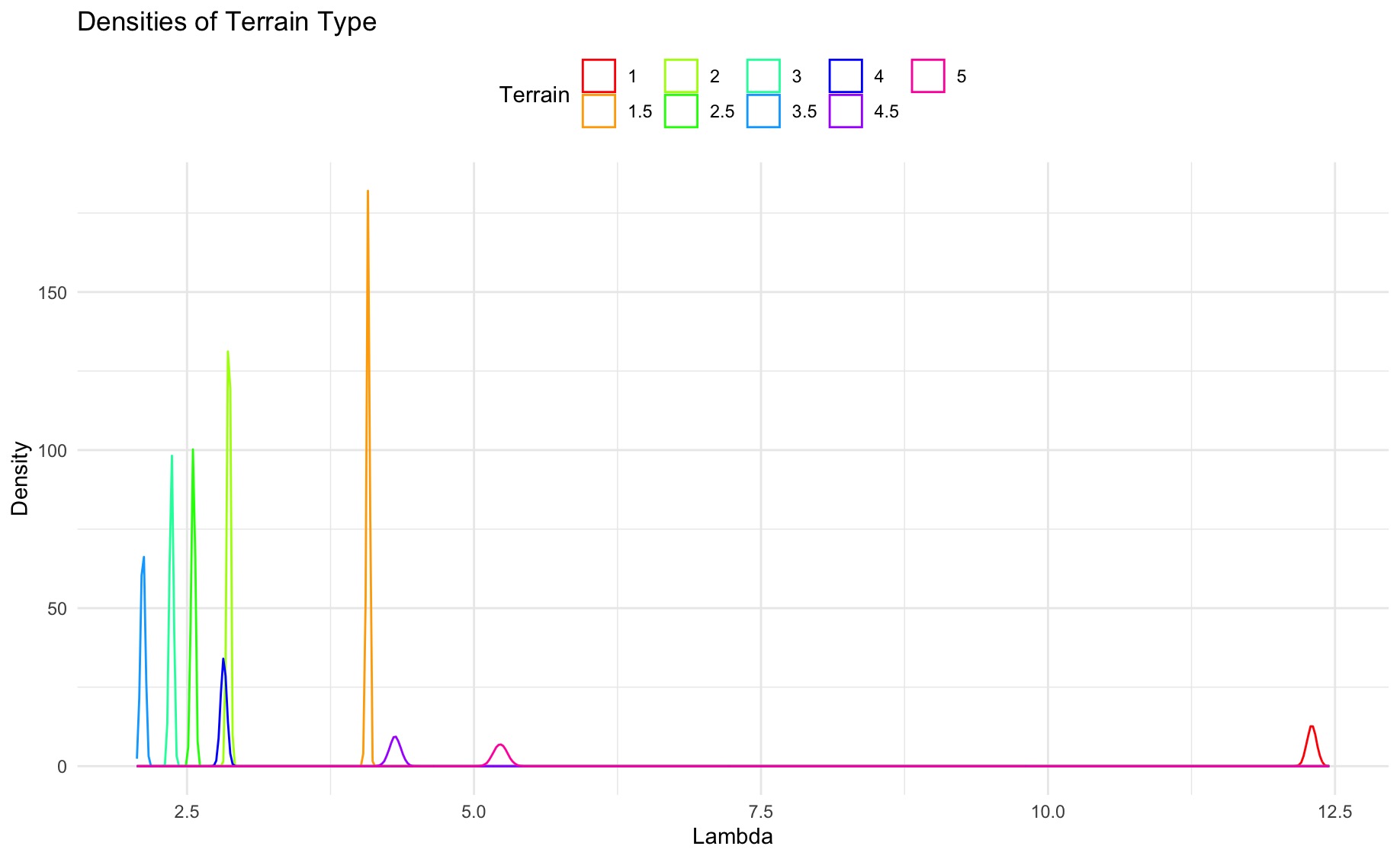
Densities of mean number of favorites by Terrain rating
Frequentist analysis
Just for fun because this was a Bayesian project, we also performed a Frequentist analysis in the form of just finding the MLE for each group. The Frequentist analysis closely mirrors the results of our Bayesian analysis, which we think is just a result of us having so much data. The nice things about the Bayesian analysis though, and the reason we chose to do it, is because of the nice Bayesian interpretations that come along with it.
| Difficulty Level | Bayesian Lower | Bayesian Upper | Frequentist |
|---|---|---|---|
| 1 | 8.3105 | 8.4326 | 8.3709 |
| 1.5 | 2.4336 | 2.4603 | 2.4472 |
| 2 | 2.9928 | 3.0254 | 3.0091 |
| 2.5 | 4.2801 | 4.3467 | 4.3130 |
| 3 | 5.1512 | 5.2386 | 5.1940 |
| 3.5 | 6.0822 | 6.2378 | 6.1602 |
| 4 | 7.0369 | 7.2340 | 7.1352 |
| 4.5 | 8.0938 | 8.4289 | 8.2625 |
| 5 | 10.2651 | 10.6396 | 10.4520 |
Conclusion
So in conclusion, if you are just dying to go and hide a geocache and get the most favorites from it, make sure to hide either a really easy cache or a really hard one. Drew and I talked about it, and we thought that maybe geocachers really liked the extremes because a lot of them are trying to keep daily caching streaks and the easy caches are great for that, or they are looking for a crazy adventure and the really hard geocaches are great for that. Who knows? If you have another hypothesis shoot me an email and let me know. Either way it is clear that the caches with the highest and lowest Terrain and Difficulty ratings receive the most favorites.
